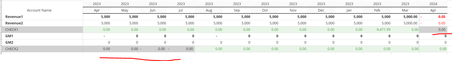
If you do a rule trace on the cells that aren’t being formatted I’m pretty sure that you will find that the value should be zero but due to floating point approximation the cell evaluates to a very small residual which is provided in scientific notation. (E.g. rather than “0.000000005678” the cell value is “5.678e-9”).
The conditional formatting in Apliqo UX doesn’t interpret the value in scientific notation as being in the defined range (in html everything is a string). This is a bug in UX which I encountered myself just this week. You can work around it in your application by applying the RoundP function in the TM1 rule for the value to round the value to a set number of decimal places.
This depends. Assuming that CHECK1 and CHECK2 are elements from a TM1 dimension then as described you need to do this in the TM1 rules for the cube which is providing the data for the view. Whatever the rule currently is for CHECK1 would be wrapped in the RoundP function.
If the check rows have been inserted in UX then you would just use the ROUND function in the formula. The same as you would in Excel.